
Regression
Linear Regression
Linear regression is the statistical method of using features (independent variables) to analyze the relationship and predict a continuous response (dependent) variable. The method creates a best-fit line (or plane in multiple linear regression) to best analyze the change in the target variable corresponding to changes in the values of feature variables. Linear regression equations come in the form of:
Where B0 is the intercept term and each X_i value is the predicted change in the response variable that occurs from a one unit increase in the corresponding B value. The model parameters are created through the analysis of a training set of data containing both feature and response values. After creation, the model is fed feature variables and predicts a response value.


Example of Logistic Regression Best-fit Line
Linear vs. Logistic Regression
As mentioned above, both linear and logistic regression models analyze the relationships between feature variables and the response variable. Furthermore, both regression techniques apply linear combinations of feature inputs, require training data, and use optimization technique to find the best fit line - such as gradient descent. However, linear regression is used to predict the value of a continuous variable where logistic regression is used to predict a binary classification and returns a probability value between 0 and 1. Furthermore, linear regression returns a straight line while logistic regression returns a sigmoid curve.

Linear regression equation and sigmoid transformation
Logistic Regression and Maximum Liklihood
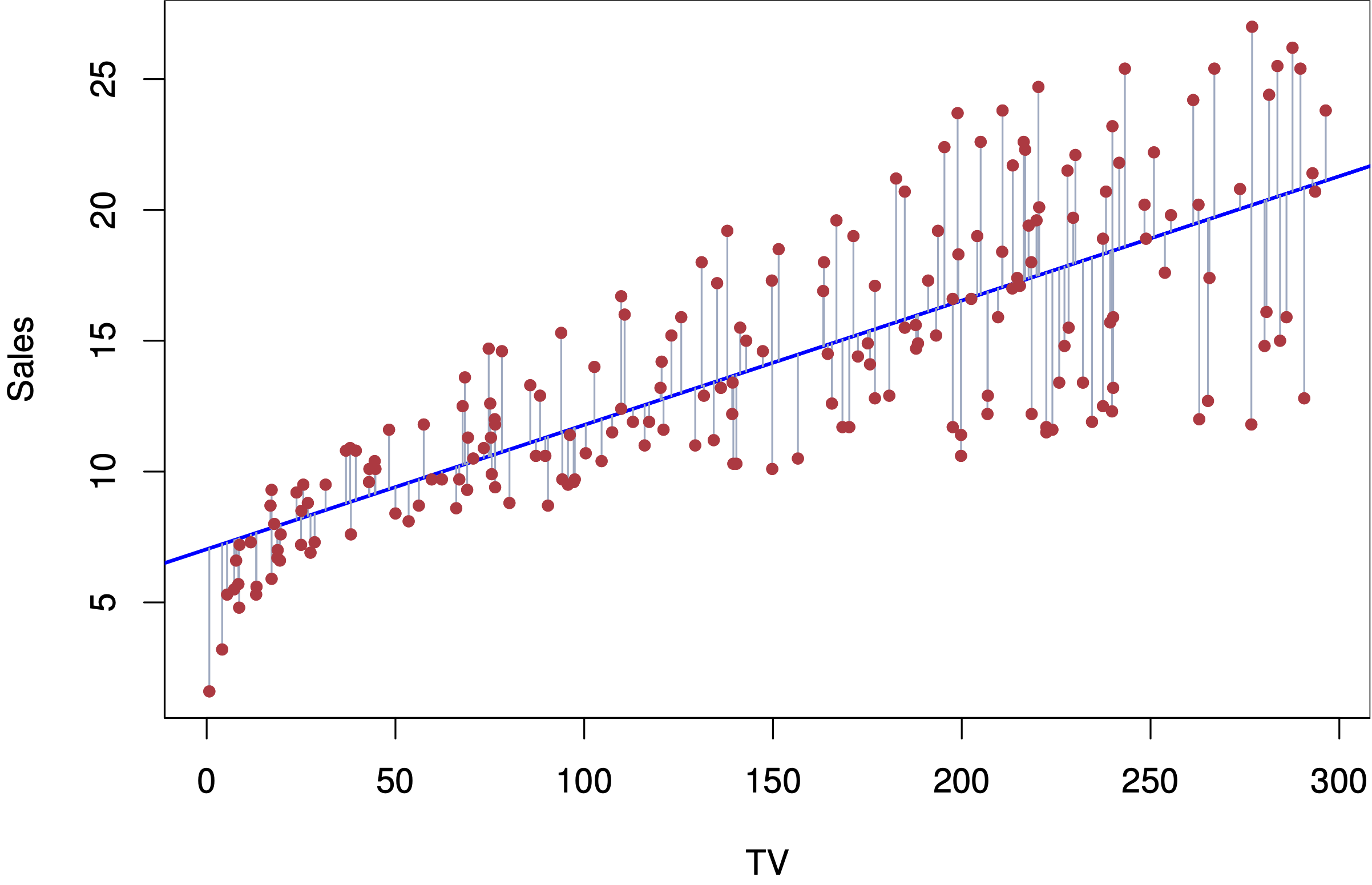
Example of Linear Regression Best-fit Line
Logistic Regression
Alternatively, logistic regression uses feature variables to predict a binary response. Through the use of the sigmoid function logistic regression converts a linear regression equation to instead return a probability between 0 and 1. This probability then in turns determines the binary output (the threshold is typically 0.5)
Logistic regression follows a similar method of model training as linear regression. The model is given feature values with the corresponding binary classification to create a best fit model and corresponding parameter values. Upon the completion of the model it is then given feature values and asked to predict the binary response.

While linear regression creates models by minimizing the error logistic regression applies Maximum Likelihood Estimation (MLE) to determine parameter values. Specifically, logistic regression maximizes the log-likelihood function to create the highest likelihood of returning a probability close to 0 when the true value is 0 and a probability close to 1 when the true value is 1.
Example of Logistic vs. Linear Regression Best-fit Lines
Logistic Regression and the Sigmoid function
One of the defining characteristics of logistic regression is the application of the sigmoid function. Logistic regression passes a linear regression equation through the sigmoid function in order to convert a continuous response into a probability outcome between 0 and 1. For example given the linear function z (right), by passing z through the sigmoid a probability value p is returned.

Likelihood and Log-likelihood functions
Logistic regression requires a labeled dataset that has only 2 categories for the data used in the analysis the label is the race distance, and will either correspond to a 50 mile (4,447 responses) or 100 kilometer (4,652 responses) race. Furthermore, the algorithm works best with continuous numeric or binary input features
After the data has been adequately prepared it must be split into a training and a test set. For the following model the training set was comprised of 80% of the responses and the model was then testes on the remaining 20% of responses. It is crucial for these two sets to be completely disjoint from one another so that the model performance can be accuratley gauged given its performance on previously unseen data.
For the below analysis the exact same orgin datset as well as trainign and test sets were used in both logistic regression and multinomial Naive Bayes

Snipit of cleaned and prepared data
Data Preparation


Snipit of training-set data
Snipit of test-set data
Comparisson of Logistic Regression and Multinomial Naive Bayes
Logistic Regression
When predicting the label for the 1,820 responses in the test set the multinomial Naive Bayes model accurately predicted the distance of the race on 81.3% of responses. The model is performing quite well but not perfectly.
More specifically by analyzing the confusion matrix the model does not have any major biases although there is a slight tendancy to over predict the shorter distance race (50 miles / 80 km). The model predicted this class for 51.7% of responses when in reality the class only made of 50% of the test set.

Confusion Matrix for Multinomial Naive Bayes

Confusion Matrix for Logistic Regression
Multinomial Naive Bayes
When predicting the label for the exact same1,820 responses in the test set the multinomial Naive Bayes model accurately predicted the distance of the race on only 72.5% of responses. This model performed had approximately a 9% worse accuracy score compared to the logistic regression analysis.
Furthermore, by examining the confusion matrix it is obvious that the bias of choosing the shorter race class is much more pronounced in the multinomial NB compared to logistic regression. The model predicted this class for 55% of responses instead of the expected 50%.
Summary of Conclusions
As discussed above, the logistic regression model far outperformed the multinomial Naive Bayes model when exaiming the exact same test and training datasets. The logistic regression model accurately predicted the test class 81.3% of the time and did not exhibit any extreme biases. However, it is important to note that the Gaussian Naive Bayes model outperformed both of the models examined here when tested on the same dataset (see the Bayesian Models tab for further info).
Given the data being examined is is likely that the logistic model performed better in part due to the multinomial NB model’s assumption of feature independence. This assumption is unlikely to be accurate given race data, for example, the hours it takes to complete a race will be correlated with the elevation gain experienced through out the course. Furthermore, logistic regression is able to learn and incorporate feature interaction when multinomial NB does not.
The logistic regression model performing better in this test suggests that ultra-running race result variables may be highly correlated with one another and exhbit powerful feature interactions. Furthermore, given that neither of the models had an accuracy score over 85% iit is likely that important features may be missing from the datas. One potential missing component could be the race course surface: is it on pavement? Grass? Sand? Rocky trails?