

Support Vector Machines
Overview
Support vector machines (SVM) are a supervised machine learning technique which will be applied in this context for binary classification. The models will attempt to determine the distance of a race result - 50 miles or 100 kilometer. SVMs are considered linear separators because they try to find a straight line between data points to enable easy classification. However, this straight line approach is onl applicable for 2-dimensional data, at higher dimensions the model creates a hyperplane to attempt to distinguish between classes.
Kernels are the primary functions that enable SVMs to build complex separators - as high-dimensional data is rarely separable by a straight line - and map data features into higher dimensional space. SVM’s apply dot products to determine the similarity and relative “closeness” between data points. Dot products are the basis for all kernels, including those of higher dimensionality, which applies a generalized dot product to a higher dimensional feature space. Two of the most common SVM kernels are the poly and rbf kernels. The polynomial kernel creates a curved decision boundary (hyperplane) following to the polynomial degree. For example the curve will resemble a parabola for a degree 2 polynomial kernel. The radial basis function (RBF) kernel, is much more complex and creates a more adaptable decision boundary which can be specific enough to wrap tightly around points if class arrangements are more complex.

Visualization of SVM mapping in higher dimensional space to separate data

Visualization of linear kernel (left) and polynomial kernel degree 2 (right)

Example of using a polynomial kernel to “cast” a 2D point into 6 dimensions
Data Prep
For each of the SVM models, labels are required to train and test the model. For the following analysis the label for the data is the race distance, and either corresponds to a 50 mile (4,447 responses) or 100 kilometer (4,652 responses) race. For best SVM performance features are numeric and continuous .
After the data has been adequately prepared it must be split into a training and a test set. For the following models the training set was comprised of 80% of the responses and the model was then testes on the remaining 20% of responses. It is crucial for these two sets to be completely disjoint from one another so that the model performance can be accurately gauged given its performance on previously unseen data.

Snipit of data to be used (above)

Snipit of training data to be used

Snipit of test data to be used
Modeling
Polynomial Degree 3 Kernel
Applying a polynomial degree 3 kernel to train SVM models resulted in the below confusion matrices and performance metric summaries. Cost parameters of 1, 10, and 0.01 were applied. As evident from the below plots and performance summaries, the degree 3 polynomial model with C = 10, outperformed the other models with lower cost parameters. This model had a correct classification accuracy of ~82%. However, all three of these polynomial models were victim to over-predicting the longer race category (100km).


Polynomial Degree 2 Kernel
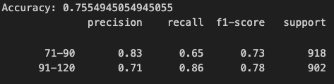
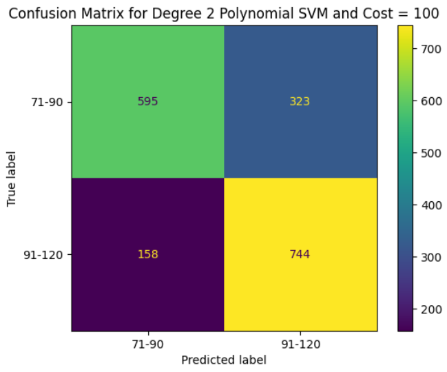
Implementing a polynomial degree 2 kernel to train SVM models created the below confusion matrices and corresponding performance outputs. Cost parameters of 1, 10, and 100 were applied. The below plots and performance summaries demonstrate, the degree 2 polynomial model with C = 10, outperformed the other models which exhibited both a higher and lower cost parameter. This model had a correct classification accuracy of ~75.5%. However, as with the polynomial degree 3 kernel, all three of these polynomial degree 2 models were victim to over-predicting the longer race category (100km).


RBF Kernel


The following confusion matrices and performance outputs are from SVM models trained with an rbf kernel. Cost parameters of 1, 10, and 100 were applied. The below outputs show that the rbf kernel models are far outperforming SVMs trained on other kernels. Again, in this instance, the model with the highest C (100) performed the best. This model had a correct classification accuracy of ~97%. Interestingly the lower cost models overpredicted the 50 mile distance, while the high cost model over-predicted the 100km race.


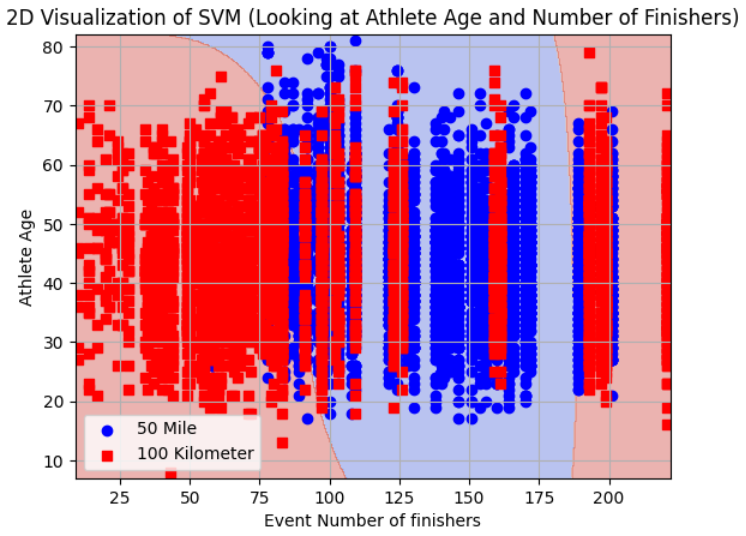
RBF Kernel - Decision Boundary 2-D Visualization


It is impossible to create a visualization which can portray how the model created a hyper plane through 6+ dimensional space. However, below are visualizations of the separator created by RBF 2 feature support vector machines. By examining these plots, the viewer can begin to understand how stacking features can lead to a very powerful classifying model - and a very complicated separator.

Summary of Conclusions
As obvious from the above model discussions, the rbf model far outperforms the polynomial models when classifying observations as either a result from a 50 mile or 100 kilometer race. This suggests that the the boundary between the two classes is highly nonlinear. The pattern within the data is too complex to be captured by the fixed curves of polynomial models. The rbf model with a cost parameter of 100 does an excellent job of predicting race distances.
This model also outperforming all naive bayes and regression models tested. When considering the utra-running dataset this makes logical sense as their are not clear linear boundaries between classes and classes are not conditionally independent - leading to poor Naive Bayes performance.